Dynamics of Structures
Structural Engineering Simplified
4.2 Numerical Solution of the Equation of Motion

Figure 4.2.1 Piecewise Linear Load
We have seen how Duhamel's integral can be very helpful in providing a closed form solution for the equation of motion. For many practical cases, the type of load is not as simple as we have seen in the previous section. In the more complex cases, numerical methods are normally used to solve the equation of motion. The method that we will present here is exact for a general loading function that can be modeled by piecewise linear segments. It will provide excellent results as long as the time step is chosen to be small enough to capture all the critical points in the loading function.
Representing the Excitation by a linear function
Any arbitrary excitation the system can be subjected to can be descritized using a picewise function as follows,
Eq. 4.2.1
Where,
Eq. 4.2.2
And,
Eq. 4.2.3
The equation of motion becomes,
Eq. 4.2.4
After some algebra, recurrence formulas for the displacment, velocity and accelerations can be obtained as follows,
Eq. 4.2.5
Eq. 4.2.6
Eq. 4.2.7
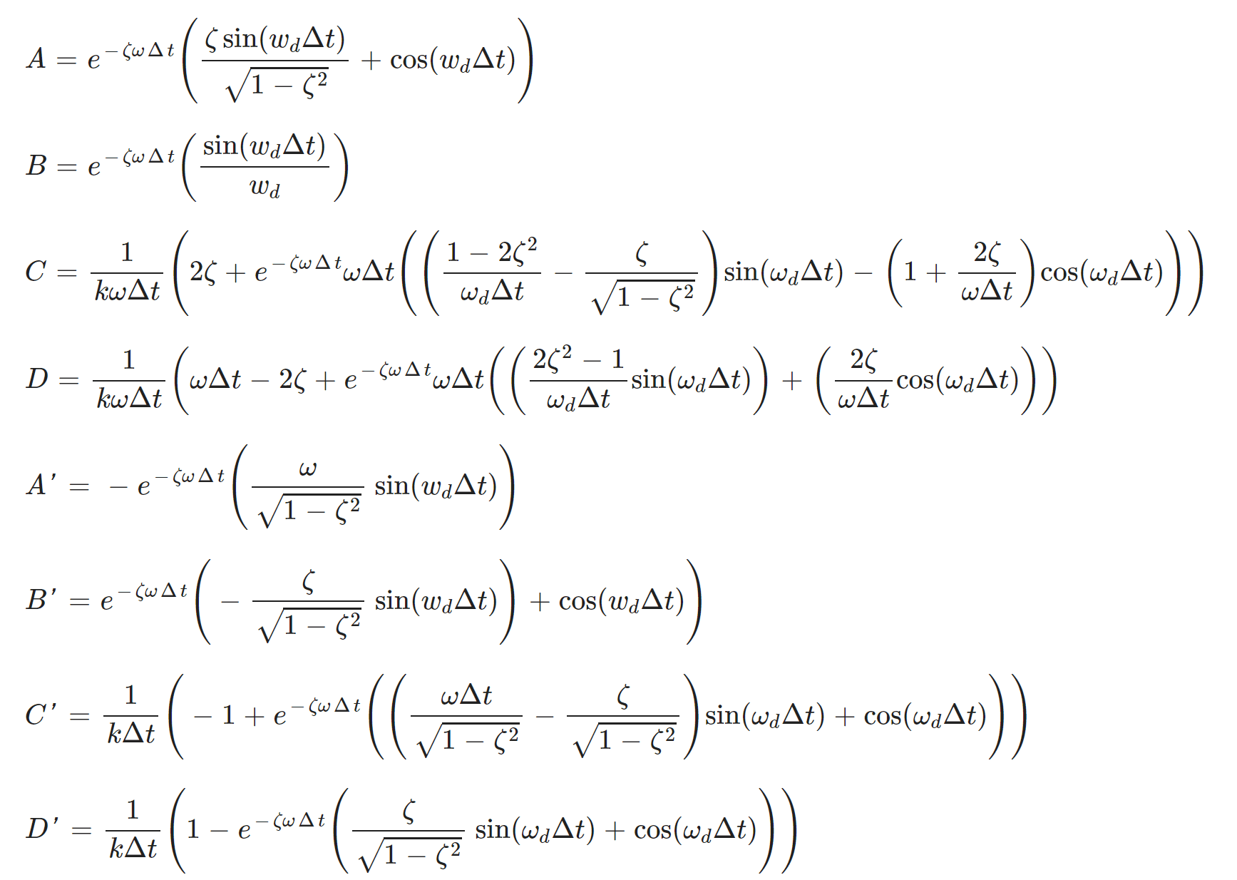
Figure 4.2.2 Constants for the Numerical Method
Application of the Numerical Method
Control Parameters
m
k
ζ
T
Select Pulse Type


Additional Control Parameters
td
Fo
Turn off or on items in the graph legend by clicking on the rectangle in the legend to adjust the scale of the graph automatically
Observations
Numerical method can be used to solve the equation of motion effectively and efficiently. The application of the method was illustrated for different pulses in the previous tool.
Other numerical methods also exist and can be reviewed in many of the available references.